Top MS Excel Formulas in Hindi? |Top MS Excel Formulas List in Hindi

आज हम आपको MS Excel top formulas with examples in Hindi PDF में सीखाएंगे। और यह Top MS Excel for Beginners के लिए भी उपयोगी है और Top MS Excel formulas pdf download भी कर सकते है जो Top MS Excel for Interview में भी काम आएंगे। और Excel Formulas A to Z List in Hindi PDF भी मिलेगी।

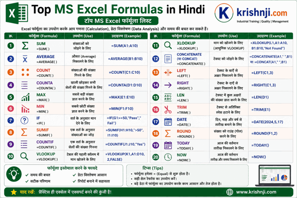
Excel Formula List A to Z in Hindi| Excel Formulas List with Examples in Hindi PDF

Formula या Function

यह क्या करता है

उपयोग का उदाहरण

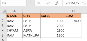
SUM()

यह संख्याओं को जोड़ने के का आता है।

=SUM(Select Numbers)

=SUM(C2:C5)

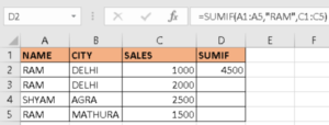
SUMIF()

Important Points

SUMIF = single condition
Text condition quotes में ” “
Different columns use कर सकते हैं
Case sensitive नहीं है

यह संख्याओं को कंडीशन के अनुसार जोड़ने के काम आता है।

=SUMIF(range, criteria,[sum range])

Argument	Meaning
range	जहाँ condition check होगी
criteria	condition
sum_range	जिनको sum करना है

SUMIFS()

Important Rules

1. SUMIFS में sum_range पहले आता है

2. Multiple conditions allowed

3. AND logic use करता है

4. Same size ranges जरूरी

यह multiple कन्डिशन में संख्याओं को जोड़ने के काम आता है।

=SUMIFS(sum_range, criteria_range1, criteria1, [criteria_range2, criteria2]…)

Argument	Meaning
sum_range	जिनको sum करना है
criteria_range1	condition range 1
criteria1	condition 1
criteria_range2	condition range 2
criteria2	condition 2

यहाँ हम दो कन्डिशन, राम की दिल्ली की कन्डिशन लगा कर sum निकाला है।

SUMIF vs SUMIFS

SUMIF	SUMIFS
single condition	multiple condition
syntax simple	syntax reversed
older	advanced

SUMPRODUCT()

यह same position के numbers का गुणा करता है और फिर सभी का total निकालता है।

=SUMPRODUCT(array1,[array2],[array3],[array4],……)

Calculation(1*1000)+(2*2000)+(5*2500)=17500

MIN()

यह संख्याओं में से सबसे छोटी संख्या को निकालने के काम आता है।

=MIN(Number1,Number2,….)

MAX()

यह संख्याओं में से सबसे बड़ी संख्या को निकालने के काम आता है।

=MAX(Number1,Number2,…..)

AVERAGE()

यह संख्याओं का औसत निकालने के काम आता है।

=AVERAGE(Number1,Number2,…)

AVERAGEIF()

यह कन्डिशन के अनुसार संख्याओं का औसत निकालने के काम आता है।

AVERAGEIFS()

यह multiple कन्डिशन में औसत निकालने के काम आता है।

COUNT()

यह संख्याओं को गिनने के काम आता है।

COUNTIF()

यह कंडीशन के अनुसार संख्याओं को गिनने के काम आता है।

COUNTIFS()

यह कई कंडीशन के अनुसार संख्याओं को गिनने के काम आता है।

COUNTA()

यह सभी रेंज को count करता है।

COUNTBLANK()

यह BLANK को गिनने के काम आता है।

CEILING()

यह किसी संख्या को ऊपर की ओर round करने के काम आता है।

=CEILING(number,significance)

=CEILING(23.4,1)

FIND() और REPLACE()

यह find और replace करने के काम आता है।

UPPER()

यह लिखे इंग्लिश शब्दों को upper case में बदल देता है।

LOWER()

यह लिखे इंग्लिश शब्दों को lower case में बदल देता है।

PROPER()

यह लिखे इंग्लिश शब्दों को proper case (अर्थात पहले लेटर को बड़ा) में बदल देता है।

CONCATENATE()

यह कई text या values को जोड़ने के काम आता है।

यह पुराना फार्मूला है।

CONCAT()

यह कई text या values को जोड़ने के काम आता है।

TEXTJOIN()

यह कई text या cell values को जोड़ने, और बीच में automatic separator लगाने के काम आता है। यह concat() और concatenate() से ज्यादा पावरफुल है।

Delimiter:- बीच में क्या लगाना है (जैसे space, comma)

text1, text2:- कौन-कौन से cell जोड़ने है।

Ignore_empty:-TRUE(खाली cell छोड़ देगा), FALSE(खाली भी छोड़ देगा)

LEFT()

यह किसी text के शुरू के left side से characters निकालने के काम आता है।

=LEFT(text, [num_chars])

text:-जिस cell से निकालने है।

num_chars:-कितने characters निकालने है।

RIGHT()

यह किसी text के शुरू के right side से characters निकालने के काम आता है।

=RIGHT(text, [num_chars])

text:-जिस cell से निकालने है।

num_chars:-कितने characters निकालने है।

MID()

यह किसी text के शुरू के middle से characters निकालने के काम आता है।

=LEFT(text, start_num,num_chars)

text:-जिस cell से निकालने है।

start_num:-कितने नंबर या character से निकालना है।

num_chars:-कितने characters निकालने है।

LEN()

यह किसी text में कितने character है यह गिनता है।

=LEN(text)

Note:- यह space को भी गिन लेता है।

SUBSTITUTE()

यह text के अंदर किसी word/character को बदलने (replace) करने के काम आता है।

=SUBSTITUTE(text,old_text,new_text,[instance_num])

text:- original text

old_text:- क्या बदलना है।

new_text:-किससे बलना है।

instance_num[optional]:-कौन से occurrence बदलना है।

NOW()

यह वर्तमान date और time बताता है।

=NOW()

TODAY()

यह वर्तमान date बताता है।

=TODAY()

TIME()

Hour,Minut,Second को मिलाकर valid time बनाना होता है।

=TIME(hour, minute, second)

Example:-

Simple time बनाना

TIME(10,30,3)

10:30AM

Current time में 2 घंटे जोड़ना

3:00AM+TIME(2,0,0)

Seconds को time में बदलना

Practical Office use

· Shift timing calculate करना

· Overtime calculate करना

· Production hour tracking

DATEDVALUE()

यह Text format में लिखी हुई लिखी हुई date को excel की real date में बदल देता है

=DATE(date_text)

YEAR()

YEAR function किसी भी date से सिर्फ वर्ष (Year) निकालने के लिए उपयोग करते है।

=YEAR(serial_number)

YEAR कब काम आता है।

ü Sales report में Year wise data निकालने के लिए

ü Age calculate करने में

ü Pivot table में year wise group करने में

ü Financial year analysis करने में

MONTH()

MONTH function किसी भी date से सिर्फ महीना निकालता है।

MONTH(serail_number)

YEAR कब काम आता है।

ü Sales report में Month wise data निकालने के लिए

ü Salary sheet में month निकालने के लिए

ü Pivot table में month wise group करने में

Financial analysis करने में

EOMONTH()

EOMONTH का मतलब है End of month. यह किसी भी date से उस महीने का आखिरी दिन (last day) निकालता है।

=EOMONTH(start_date,months)

ü start_date:-कोई भी डेट

ü months:-कितने महीने आगे/पीछे जाना है।

ü 0=उसे महीने का last day

ü 1=अगले महीने का last day

ü -1=पिछले महीने का last day

YEAR कब काम आता है।

ü Salary calculation

ü EMI due date planning

ü Financial report closing

ü GST/monthly report

WEEKDAYS()

WEEKDAY function किसी भी Date से बताता है कि वह कौन-सा दिन (Monday, Tuesday आदि) है — लेकिन number के रूप में।

=WEEKDAY(serial_number, [return_type])

serial_number → Date वाली cell
return_type → Week की गिनती कहाँ से शुरू करनी है

Return Type समझो (Important)

return_type	Week Start	Result Range
1 (default)	Sunday	1 = Sunday, 7 = Saturday
2	Monday	1 = Monday, 7 = Sunday
3	Monday	0 = Monday, 6 = Sunday

NOTE:- India में आमतौर पर 2 use करना बेहतर है।

Weekend Check Formula

अगर Monday = 1 system (return_type 2) use कर रहे हो:

=IF(WEEKDAY(A1,2)>5,”Weekend”,”Working Day”)

Practical Use

✔ Salary sheet में Sunday identify करने के लिए
✔ Attendance system
✔ Weekend detect करने के लिए
✔ Auto holiday highlight (Conditional Formatting)

DATE()

DATE function से आप Year, Month और Day देकर एक सही (Real) Date बना सकते हो।

=DATE(year, month, day)

year → साल
month → महीना (1–12)
day → दिन (1–31)

=DATE(2026,3,1)

Result: 01-03-2026

Example 2 (Cell Reference से)

अगर
A1 = 2026
B1 = 3
C1 = 15

तो formula:

=DATE(A1,B1,C1)

Result: 15-03-202

DATE कब काम आता है?

✔ जब Year, Month, Day अलग-अलग columns में हो
✔ Financial Year calculation
✔ Report automation
✔ Text date error avoid करने के लिए

Text date की problem खत्म (VLOOKUP / MATCH में error नहीं)

✔ Month > 12 या Day > 31 होने पर भी Excel auto adjust कर देता है

=DATE(2026,13,1) → 01-01-2027

✔ Age, EMI, Salary, Report में calculation smooth

Practical Office Use

Current date से next month बनाना:

=DATE(YEAR(A1),MONTH(A1)+1,DAY(A1))

Financial Year Start (India):

=DATE(YEAR(A1),4,1)

Important

अगर Date text में है (जैसे “01-03-2026”), तो पहले DATEVALUE से convert करो।

DATEDIF()

DATEDIF का मतलब है Date Difference
यह दो तारीखों के बीच का फर्क (Year, Month या Day में) निकालता है।⚠ यह function Excel में hidden है — Formula list में नहीं दिखता, लेकिन काम करता है।

=DATEDIF(start_date, end_date, unit)

start_date → शुरुआत की तारीख
end_date → अंत की तारीख
unit → किसमें फर्क चाहिए

Unit Options

Unit	Meaning	Example Result
“Y”	पूरे साल	5 Years
“M”	पूरे महीने	62 Months
“D”	पूरे दिन	1890 Days
“YM”	साल हटाकर बचे महीने	2 Months
“MD”	महीने हटाकर बचे दिन	10 Days
“YD”	साल हटाकर बचे दिन	70 Days

Example

अगर A1 = 01-03-2000
और B1 = 01-03-2026

Age (Years में)

=DATEDIF(A1,B1,”Y”)

Result: 26

Practical Use

✔ Age calculation
✔ Service period निकालना
✔ Loan duration
✔ Experience calculate करना

Professional Age Formula (Complete Format)

=DATEDIF(A1,B1,”Y”)&” Years “&DATEDIF(A1,B1,”YM”)&” Months “&DATEDIF(A1,B1,”MD”)&” Days”

Output: 26 Years 0 Months 0 Days

LOOKUP()

lOOKUP function का उपयोग किसी value को ढूँढने और उसके सामने वाली value निकालने के लिए किया जाता है।
यह पुराने version का function है — आजकल ज़्यादातर लोग VLOOKUP / HLOOKUP / XLOOKUP इस्तेमाल करते हैं।

=LOOKUP(lookup_value, lookup_vector, result_vector)

lookup_value → जो value ढूँढनी है
lookup_vector → जहाँ ढूँढना है (एक column या row)
result_vector → जिसके सामने वाली value निकालनी है

Example

मान लो:

A (ID)	B (Name)
101	Anshu
102	Rohit
103	Amit

Formula:

=LOOKUP(102,A2:A4,B2:B4)

Result: Rohit

Important Rule

✔ Lookup column Ascending Order (छोटे से बड़े) में होना चाहिए
✔ Exact match नहीं मिले तो यह छोटी नज़दीकी value पकड़ लेता है

इसलिए यह थोड़ा risky हो सकता है।

Practical Use

✔ Grade system
✔ Commission slab
✔ Approximate value find करना
✔ Simple table lookup

Difference समझो

Function	Match Type	Order Required
LOOKUP	Approximate	Yes (Ascending)
VLOOKUP	Exact + Approx	No (Exact में)
XLOOKUP	Advanced	No

VLOOKUP()

Microsoft Excel में VLOOKUP एक बहुत प्रसिद्ध फ़ॉर्मूला है। इसका उपयोग किसी टेबल में एक वैल्यू खोजकर उससे जुड़ी दूसरी जानकारी निकालने के लिए किया जाता है।

और यहाँ V का मतलब vertical होता है

=VLOOKUP(lookup_value, table_array, col_index_num, [range_lookup])

मतलब:

Parameter	मतलब
lookup_value	जो वैल्यू आप ढूंढना चाहते हैं
table_array	जिस टेबल में खोज करनी है
col_index_num	किस कॉलम से रिज़ल्ट चाहिए
range_lookup	TRUE (Approximate) या FALSE (Exact match)

आसान उदाहरण

मान लो यह टेबल है:

A (ID)	B (Name)	C (Salary)
101	Ravi	20000
102	Mohan	25000
103	Sita	30000

अगर ID 102 का Name निकालना है

=VLOOKUP(102, A2:C4, 2, FALSE)

Result: Mohan

समझो कैसे:

102 को कॉलम A में ढूंढेगा
उसी row का 2nd column (Name) देगा

Important Rules

✔ VLOOKUP हमेशा पहले कॉलम में search करता है
✔ Right side का data ही निकाल सकता है
✔ Exact match के लिए FALSE लिखना बेहतर है

Common Error

#N/A Error
जब lookup value टेबल में नहीं मिलती।

Example:

=VLOOKUP(105, A2:C4, 2, FALSE)

क्योंकि 105 मौजूद नहीं है।

HLOOKUP()

Microsoft Excel में HLOOKUP का मतलब है Horizontal Lookup।
यह टेबल की पहली row में वैल्यू खोजकर नीचे की row से डेटा निकालता है।यहाँ H का मतलब Horizontal है

=HLOOKUP(lookup_value, table_array, row_index_num, [range_lookup])

Parameter	मतलब
lookup_value	जो वैल्यू खोजनी है
table_array	पूरी टेबल
row_index_num	किस row से रिज़ल्ट चाहिए
range_lookup	TRUE (approximate) या FALSE (exact)


VLOOKUP	Vertical (Column में search)
HLOOKUP	Horizontal (Row में search)

*IMPORTANT Points

✔ HLOOKUP पहली row में search करता है
✔ नीचे की rows से data निकालता है
✔ Exact match के लिए FALSE use करें

XLOOKUP()

Microsoft Excel में XLOOKUP एक नया और बहुत powerful formula है।
यह VLOOKUP और HLOOKUP दोनों की जगह इस्तेमाल किया जा सकता है।

=XLOOKUP(lookup_value, lookup_array, return_array, [if_not_found], [match_mode], [search_mode])

lookup_value

जो वैल्यू ढूंढनी है

lookup_array

जिस column/row में search करना है

return_array

जिस column/row से result चाहिए

if_not_found

value ना मिले तो क्या दिखाना है

match_mode

exact या approximate match

search_mode

ऊपर से या नीचे से search

A (ID)	B (Name)	C (Salary)
101	Ravi	20000
102	Mohan	25000
103	Sita	30000

अगर ID 102 का Name निकालना है

=XLOOKUP(102, A2:A4, B2:B4)

Result: Mohan

अगर value ना मिले तो

=XLOOKUP(105, A2:A4, B2:B4, “Not Found”)

Result: Not Found

XLOOKUP क्यों बेहतर है

Feature	VLOOKUP	XLOOKUP
Left side lookup	❌	✅
Error handling	❌	✅
Exact match default	❌	✅
Column number	जरूरी	नहीं देना

MATCH()

Microsoft Excel में MATCH formula का उपयोग किसी वैल्यू की position (स्थान) खोजने के लिए किया जाता है।
यह बताता है कि कोई वैल्यू किस नंबर की position पर है।

=MATCH(lookup_value, lookup_array, [match_type])

Parameter	मतलब

lookup_value

जो वैल्यू खोजनी है

lookup_array

जिस range में search करना है

match_type

0 = Exact match, 1 = Less than, -1 = Greater than

आसान उदाहरण

A
Ravi
Sham
Sita
Ram

अगर Sham की position निकालनी है

=MATCH(“Sham”, A1:A4, 0)

Result: 2

MATCH + INDEX (बहुत powerful)

=INDEX(B1:B4, MATCH(102, A1:A4, 0))

इससे ID 102 का Name निकल सकता है।

* Important Points

✔ MATCH सिर्फ position बताता है
✔ Actual value निकालने के लिए INDEX के साथ use होता है
✔ Exact match के लिए 0 use करें

INDEX()

Microsoft Excel में INDEX formula का उपयोग किसी टेबल या range में से किसी खास position की value निकालने के लिए किया जाता है।

=INDEX(array, row_num, [column_num])

array – data की range

row_num – कौन सी row

column_num – कौन सा column

DGET()

Microsoft Excel में DGET formula का उपयोग Database table से किसी एक specific record की value निकालने के लिए किया जाता है, जब कुछ criteria (शर्त) दी जाती है।

=DGET(database, field, criteria)

database- पूरी data table

field- किस column से value चाहिए

criteria- किस condition पर data चाहिए

A	B	C
ID	Name	Salary
101	Ravi	20000
102	Mohan	25000
103	Sita	30000

Criteria Table

E	F
ID	102

Formula

=DGET(A1:C4, “Salary”, E1:E2)

Result: 25000

मतलब:

Table A1:C4 में search करेगा
ID = 102 ढूंढेगा
Salary column की value देगा

* Important Rule

✔ Criteria header के साथ होना चाहिए
✔ Result सिर्फ एक record होना चाहिए
✔ अगर एक से ज्यादा record मिले तो #NUM! error आएगा

*DGET कब उपयोग होता है

Database type Excel sheets
Filter करके single record निकालने के लिए
Advanced Excel reports में

DSUM

Criteria के आधार पर Sum (जोड़) निकालता है।

=DSUM(database, field, criteria)

Example Table

ID	Name	Salary
101	Ravi	20000
102	Mohan	25000
103	Ravi	30000

Criteria

Name

Ravi

Formula

=DSUM(A1:C4,”Salary”,E1:E2)

Result: 50000
(क्योंकि Ravi की Salary 20000 + 30000)

DCOUNT

Criteria के आधार पर numeric cells की गिनती करता है।

=DCOUNT(database, field, criteria)

Example Table

ID	Name	Salary
101	Ravi	20000
102	Mohan	25000
103	Ravi	30000

Example:

=DCOUNT(A1:C4,”Salary”,E1:E2)

Result: 3

DAVERAGE

Criteria के अनुसार Average निकालता है।

=DAVERAGE(database, field, criteria)

Example Table

ID	Name	Salary
101	Ravi	20000
102	Mohan	25000
103	Ravi	30000

Example

=DAVERAGE(A1:C4,”Salary”,E1:E2)

Result: 25000

DMAX

Criteria के अनुसार सबसे बड़ी value निकालता है।

=DMAX(database, field, criteria)

DMIN

Criteria के अनुसार सबसे छोटी value निकालता है।

=DMIN(database, field, criteria)

DCOUNTA

non-empty cells की गिनती करता है।

=DCOUNTA(database, field, criteria)

DSTDEV / DSTDEVP

Standard Deviation निकालता है।

=DSTDEV(database, field, criteria)

DVAR / DVARP

Variance निकालता है।

=DVAR(database, field, criteria)

VSTACK()

Microsoft Excel में VSTACK एक नया Dynamic Array formula है।
इसका उपयोग कई ranges या tables को ऊपर-नीचे (vertical) जोड़ने के लिए किया जाता है।

=VSTACK(array1, [array2], [array3], …)

Parameter	मतलब
array1	पहला data range
array2	दूसरा range
array3	तीसरा range (optional)

TABLE 1

A B

101 RAM

102 SHYAM

TABLE 2

A B

103 MOHAN

104 SOHAN

Formula

=VSTACK(A1:B3, A5:B7)

Result (दोनों tables एक साथ)

A B

101 RAM

102 SHYAM

103 MOHAN

104 SOHAN

Multiple Tables जोड़ना

=VSTACK(A1:B3, D1:E3, G1:H3)

तीनों tables एक साथ merge हो जाएँगे।

*VSTACK कहाँ काम आता है

✔ अलग-अलग sheets का data जोड़ना
✔ Monthly reports combine करना
✔ Multiple tables merge करना

Important बात

अगर columns बराबर नहीं होंगे तो Excel खाली जगह में #N/A दिखा सकता है।

HSTACK

Microsoft Excel में HSTACK एक Dynamic Array formula है।
इसका उपयोग कई ranges या tables को side-by-side (horizontal) जोड़ने के लिए किया जाता है।

=HSTACK(array1, [array2], [array3], …)

TABLE 1

A B

101 RAM

102 SHYAM

TABLE 2

D E

2000 DELHI

2500 AGRA

=HSTACK(A1:B3, D1:E3)

A B D E

101 RAM 2000 DELHI

102 SHYAM 2500 AGRA

VSTACK और HSTACK में फर्क

Formula	काम
VSTACK	Data को ऊपर-नीचे जोड़ता है
HSTACK	Data को दाएँ-बाएँ जोड़ता है

Important बात

अगर rows बराबर नहीं होंगी तो खाली जगह में #N/A आ सकता है।

FILTER

Microsoft Excel में FILTER formula का उपयोग किसी data range में से condition के अनुसार data निकालने के लिए किया जाता है।
यह automatic filtered result दिखाता है।

=FILTER(array, include, [if_empty])

Parameter	मतलब
array	पूरा data range
include	condition
if_empty	अगर data ना मिले तो क्या दिखाना है

आसान उदाहरण

A	B	C
ID	Name	Salary
101	Ravi	20000
102	Mohan	25000
103	Ravi	30000

अगर Ravi का data निकालना है

=FILTER(A2:C4, B2:B4=”Ravi”)

*RESULT

ID	Name	Salary
101	Ravi	20000
103	Ravi	30000

*FILTER formula Modern Excel का बहुत powerful tool है क्योंकि:

✔ Auto update होता है
✔ Multiple conditions लगा सकते हैं
✔ Pivot table जैसा result जल्दी देता है

UNIQUE

Microsoft Excel में UNIQUE formula का उपयोग data में से duplicate values हटाकर सिर्फ unique values निकालने के लिए किया जाता है।

=UNIQUE(array, [by_col], [exactly_once])

Parameter	मतलब
array	data range
by_col	column के अनुसार unique निकालना (TRUE/FALSE)
exactly_once	जो value सिर्फ एक बार हो वही दिखाना

आसान उदाहरण

A
Ravi
Mohan
Ravi
Sita
Mohan

UNIQUE(A1:A5)

Result

A
Ravi
Mohan
Sita

*UNIQUE formula बहुत काम आता है:

✔ Duplicate हटाने में
✔ Data cleaning में
✔ Reports बनाने में
✔ Dashboard में

SORT

Microsoft Excel में SORT formula का उपयोग data को automatically ascending या descending order में sort करने के लिए किया जाता है।
यह Dynamic Array formula है, इसलिए result auto update होता रहता है।

=SORT(array, [sort_index], [sort_order], [by_col])

Parameter		मतलब
array		data range
sort_index		किस column से sort करना है
sort_order		1 = Ascending, -1 = Descending
by_col		column के अनुसार sort (TRUE/FALSE)
A
Ravi
Ram
Sita
Amit

Formula

=SORT(A1:A4)

Result (Alphabet order)

A
Amit
Mohan
Ravi
Sita

*SORT formula बहुत काम आता है:

✔ Reports बनाने में
✔ Data analysis में
✔ Dynamic dashboards में

SORTBY

Microsoft Excel में SORTBY formula का उपयोग किसी data range को किसी दूसरे column या row के आधार पर sort करने के लिए किया जाता है।
यह SORT से ज्यादा flexible है।

=SORTBY(array, by_array1, [sort_order1], [by_array2], [sort_order2])

Parameter	मतलब
array	जिस data को sort करना है
by_array1	जिस column से sort करना है
sort_order1	1 = Ascending, -1 = Descending
by_array2	दूसरा column (optional)

आसान उदाहरण

A	B
Ravi	20000
Mohan	25000
Sita	15000

TAKE/DROP

DROP कब उपयोग करें

✔ Header हटाने में
✔ Last row हटाने में
✔ Extra columns हटाने में
✔ Dynamic reports में

Microsoft Excel में DROP formula का उपयोग range से ऊपर/नीचे या बाएँ/दाएँ से कुछ rows या columns हटाने के लिए किया जाता है।

=DROP(array, rows, [columns])

Parameter		मतलब
array		data range
rows		कितनी rows हटानी हैं
columns		कितने columns हटाने हैं
A
ID
101
102
103

अगर पहली row हटानी है:

=DROP(A1:A4,1)

👉 Result

A
101
102
103

CHOOSECOLS

CHOOSECOLS कब उपयोग करें

✔ सिर्फ जरूरी columns निकालना
✔ column order बदलना
✔ dashboard बनाना
✔ FILTER के साथ use करना

Microsoft Excel में CHOOSECOLS formula का उपयोग किसी table में से सिर्फ चुने हुए columns निकालने के लिए किया जाता है।

=CHOOSECOLS(array, col_num1, [col_num2], …)

Parameter	मतलब
array	पूरा data range
col_num1	पहला column
col_num2	दूसरा column
…	और columns

उदाहरण

A	B	C
ID	Name	Salary
101	Ravi	20000
102	Mohan	25000

अगर सिर्फ Name और Salary चाहिए

=CHOOSECOLS(A1:C3, 2, 3)

Name	Salary
Ravi	20000
Mohan	25000

CHOOSEROWS()

CHOOSEROWS कब काम आता है

✔ specific rows निकालना
✔ Top / Bottom rows लेना
✔ Dashboard बनाना
✔ FILTER के साथ use करना

Microsoft Excel में CHOOSEROWS formula का उपयोग किसी table में से सिर्फ चुनी हुई rows निकालने के लिए किया जाता है।
यह CHOOSECOLS जैसा ही है, लेकिन rows के लिए।

=CHOOSEROWS(array, row_num1, [row_num2], …)

Parameter	मतलब
array	पूरा data range
row_num1	पहली row
row_num2	दूसरी row

आसान उदाहरण

ID	Name	Salary
101	Ravi	20000
102	Mohan	25000
103	Sita	30000

अगर 1st और 3rd row चाहिए

=CHOOSEROWS(A1:C4, 1, 3)

ID	Name	Salary
ID	Name	Salary
102	Mohan	25000

NETWORKDAYS()

NETWORKDAYS कब काम आता है-

ü Salary working days

ü Attendance calculation

ü Project duration

ü Office working days

Important Points

✔ Saturday-Sunday automatically exclude
✔ holidays manually add कर सकते हैं
✔ date format सही होना चाहिए

Microsoft Excel में NETWORKDAYS formula का उपयोग दो तारीखों के बीच working days (Saturday-Sunday छोड़कर) निकालने के लिए किया जाता है।

=NETWORKDAYS(start_date, end_date, [holidays])

Parameter	मतलब
start_date	शुरू की तारीख
end_date	खत्म की तारीख
holidays	छुट्टियों की list (optional)

आसान उदाहरण

A	B
Start	End
01-01-24	10-01-24

=NETWORKDAYS(A2,B2)

Result: 8 (Saturday-Sunday हटाकर)

NETWORKDAYS.INTL()

Real use

Gulf country (Fri-Sat off)
Shift duty
Custom office calendar
Attendance sheet

Microsoft Excel में NETWORKDAYS.INTL() formula का उपयोग custom weekend के साथ working days निकालने के लिए किया जाता है।
यह NETWORKDAYS का advanced version है।

=NETWORKDAYS.INTL(start_date, end_date, [weekend], [holidays])

Parameter		मतलब
start_date		शुरू की तारीख
end_date		खत्म की तारीख
weekend		कौन से दिन छुट्टी
holidays		extra holidays (optional)
Code	Weekend
1	Saturday, Sunday
2	Sunday, Monday
3	Monday, Tuesday
4	Tuesday, Wednesday
5	Wednesday, Thursday
6	Thursday, Friday
7	Friday, Saturday
Formula			Weekend
NETWORKDAYS			Fixed (Sat-Sun)
NETWORKDAYS.INTL			Custom weekend

WORKDAY()

Real use

✔ Delivery date calculate
✔ Project deadline
✔ Leave end date
✔ Working day planning

Microsoft Excel में WORKDAY formula का उपयोग किसी तारीख में working days जोड़कर नई तारीख निकालने के लिए किया जाता है।
यह Saturday-Sunday को छोड़कर days जोड़ता है।

=WORKDAY(start_date, days, [holidays])

Parameter	मतलब
start_date	शुरू की तारीख
days	कितने working days जोड़ने हैं
holidays	छुट्टियाँ (optional)

WORKDAY vs NETWORKDAYS

Formula	काम
WORKDAY	Date निकालता है
NETWORKDAYS	Days गिनता है

DATEDIF()

Microsoft Excel में Age निकालने के कई तरीके हैं, लेकिन सबसे सही तरीका DATEDIF formula है।

Years में Age निकालना

अगर Date of Birth A1 में है

=DATEDIF(A1,TODAY(),”Y”)

Result: पूरी उम्र (years में)

Years + Months + Days (Full Age)

=DATEDIF(A1,TODAY(),”Y”)&” Years “&DATEDIF(A1,TODAY(),”YM”)&” Months “&DATEDIF(A1,TODAY(),”MD”)&” Days”

Result:
25 Years 3 Months 10 Days

सिर्फ Months में Age

=DATEDIF(A1,TODAY(),”M”)

Total months

सिर्फ Days में Age

=DATEDIF(A1,TODAY(),”D”)

Total days

TRIM()

TRIM कब use करें

✔ Copy-paste data clean करना
✔ VLOOKUP error fix करना
✔ Import data clean करना
✔ Extra spaces हटाना

Microsoft Excel में TRIM formula का उपयोग extra spaces हटाने के लिए किया जाता है।
यह text के बीच का एक space छोड़कर बाकी सभी extra spaces हटा देता है।

=TRIM(text)

Parameter	मतलब
text	जिस text से extra spaces हटानी हैं

TRIM + CLEAN (Best combo)

=TRIM(CLEAN(A1))

Hidden spaces + extra spaces दोनों हटेंगे

TRIMMAEN()

TRIMMEAN कब use करें

✔ Outliers हटाना
✔ Survey data
✔ Salary analysis
✔ Marks analysis

Microsoft Excel में TRIMMEAN formula का उपयोग average निकालने के लिए किया जाता है लेकिन extreme values (top & bottom) हटाकर।
मतलब outliers हटाकर average निकालता है।

=TRIMMEAN(array, percent)

Parameter	मतलब
array	data range
percent	कितना % data हटाना है

TRIMMEAN vs AVERAGE

Formula	काम
AVERAGE	सबका average
TRIMMEAN	extreme हटाकर average

MODE()

Microsoft Excel में MODE formula का उपयोग सबसे ज्यादा बार आने वाली value निकालने के लिए किया जाता है।
इसे Most frequent value कहते हैं।

=MODE(number1, [number2], …)

या

=MODE.SNGL(range)

MODE vs AVERAGE vs MEDIAN

Formula	मतलब
AVERAGE	average
MEDIAN	बीच की value
MODE	सबसे ज्यादा आने वाली

SMALL()

Microsoft Excel में SMALL formula का उपयोग list में से smallest value निकालने के लिए किया जाता है।
मतलब सबसे छोटा, दूसरा छोटा, तीसरा छोटा आदि।

=SMALL(array, k)

Parameter	मतलब
array	data range
k	कौन-सा smallest चाहिए

SMALL vs LARGE

Formula	काम
SMALL	smallest value
LARGE	largest value

=LARGE(array, k)

RANK.AVG()

Microsoft Excel में RANK.AVG formula का उपयोग numbers को rank देने के लिए किया जाता है, और tie होने पर average rank देता है।

=RANK.AVG(number, ref, [order])

Parameter	मतलब
number	जिस value का rank चाहिए
ref	पूरी range
order	0 = descending, 1 = ascending

RANK vs RANK.AVG

Formula	Tie case
RANK	same rank देता है
RANK.AVG	average rank देता है

IF()

Microsoft Excel में IF formula का उपयोग condition check करके result देने के लिए किया जाता है।
अगर condition सही- value 1अगर गलत-value 2

=IF(logical_test, value_if_true, value_if_false)

Parameter	मतलब
logical_test	condition
value_if_true	सही होने पर
value_if_false	गलत होने पर

आसान उदाहरण

Marks = 60
Pass mark = 50

=IF(A1>=50,”Pass”,”Fail”)

Result: Pass

IFS()

Uses

IFS ज्यादा readable
✔ आसान लिखना
✔ multiple condition easy

Microsoft Excel में IFS formula का उपयोग multiple conditions check करने के लिए किया जाता है।
यह Nested IF का आसान version है।

=IFS(condition1, result1, condition2, result2, condition3, result3…)

Marks	Grade
85	A
70	B
50	C
30	Fail

=IFS(A1>=80,”A”, A1>=60,”B”, A1>=40,”C”, A1<40,”Fail”)

IFS vs IF

Nested IF:

=IF(A1>=80,”A”,IF(A1>=60,”B”,IF(A1>=40,”C”,”Fail”)))

IFS:

=IFS(A1>=80,”A”,A1>=60,”B”,A1>=40,”C”,A1<40,”Fail”)

Important note

IFS में last condition देना जरूरी है

Example:

=IFS(A1>=80,”A”,A1>=60,”B”,TRUE,”Fail”)

OR()

Microsoft Excel में OR formula का उपयोग multiple conditions में से कोई एक सही हो तो TRUE देने के लिए किया जाता है।

👉 एक भी condition सही = TRUE
👉 सभी गलत = FALSE

=OR(logical1, logical2, …)

आसान उदाहरण

=OR(A1>50,B1>50)

अगर A1 या B1 में से कोई भी 50 से बड़ा है → TRUE

IF + OR (सबसे ज्यादा use)

=IF(OR(A1>=50,B1>=50),”Pass”,”Fail”)

किसी एक subject में pass → Pass

OR vs AND

Formula	Result
OR	कोई एक सही
AND	सभी सही

AND()

Important Points

✔ AND का result सिर्फ TRUE / FALSE होता है
✔ IF के साथ ज्यादा use होता है
✔ सभी condition सही होना जरूरी

Excel में AND फ़ॉर्मूला का उपयोग तब होता है जब एक से ज़्यादा शर्तें (conditions) एक साथ check करनी हों और result तभी TRUE आए जब सभी शर्तें सही हों

=AND(logical1, logical2, …)

Example : दो शर्त check करना

अगर A1 में marks और B1 में attendance है
पास तभी जब marks ≥ 40 और attendance ≥ 75

=AND(A1>=40,B1>=75)

✔ दोनों सही → TRUE
कोई एक गलत → FALSE

Example : AND + IF (सबसे ज्यादा उपयोग)

=IF(AND(A1>=40,B1>=75),”PASS”,”FAIL”)

Result: PASS या FAIL

AND+OR()

याद रखने की ट्रिक

AND = सब सही होना चाहिए
OR = कोई एक सही हो
दोनों मिलाकर = कुछ जरूरी + कुछ optional

Excel में AND + OR एक साथ तब इस्तेमाल होता है जब कुछ conditions जरूरी हों और कुछ में विकल्प (option) हो।

=IF(AND(Condition1, OR(Condition2,Condition3)),”Yes”,”No”)

मतलब:

Condition1 जरूरी
Condition2 या Condition3 में से कोई एक

Example (Marks + Subject)

Student PASS अगर:

Marks ≥ 40 और
Subject Math या Science हो

=IF(AND(A1>=40,OR(B1=”Math”,B1=”Science”)),”PASS”,”FAIL”)

उल्टा (OR के अंदर AND)

अगर ये condition हो:

(Math ≥ 40 AND English ≥ 40)
या
Sports = Yes

=IF(OR(AND(A1>=40,B1>=40),C1=”Yes”),”PASS”,”FAIL”)

NOT()

Common Use

✔ “Not equal to” के लिए
✔ “Except” condition
✔ Absent / No / Blank check

Excel में NOT फ़ॉर्मूला का मतलब होता है उल्टा करना (Reverse)

TRUE → FALSE
FALSE → TRUE

=NOT(logical)

Example 1

=NOT(A1>50)

अगर A1 = 60
तो A1>50 = TRUE
NOT → FALSE

Example 2 (IF + NOT)

Marks 40 से कम हों तो FAIL

=IF(NOT(A1>=40),”FAIL”,”PASS”)

XOR()

Excel में XOR फ़ॉर्मूला का मतलब है — केवल एक condition सही हो
अगर दोनों सही या दोनों गलत → FALSE

=XOR(logical1, logical2, …)

XOR vs OR vs AND

Formula	कब TRUE
AND	सभी सही
OR	कोई एक सही
XOR	केवल एक सही

ISBLANK()

ISBLANK check करता है कि cell खाली है या नहीं।

=ISBLANK(value)

अगर cell खाली है → TRUE
अगर cell में कुछ भी है → FALSE

ISEVEN()

ISEVEN check करता है कि number Even (सम संख्या) है या नहीं।

=ISEVEN(number)

Even number → TRUE
Odd number → FALSE

ISODD()

ISODD check करता है कि number Odd (विषम संख्या) है या नहीं।

Odd number → TRUE
Even number → FALSE

=ISODD(number)

Odd number → TRUE

Even number → FALSE

ISNUMBER()

ISNUMBER check करता है कि value number है या नहीं।

Number → TRUE
Text / blank / error → FALSE

=ISNUMBER(value)

ISERROR()

ISERROR check करता है कि formula में error है या नहीं।

Error → TRUE
No error → FALSE

=ISERROR(value)

Error → TRUE
No error → FALSE

TRANSPOSE()

TRANSPOSE rows को columns में और columns को rows में बदल देता है।

=TRANSPOSE(array)

array → वो range जिसे आप flip करना चाहते हैं

Note: TRANSPOSE एक array formula है। Excel 365/2021 में सीधे ENTER, पुराने version में Ctrl+Shift+Enter देना पड़ता है।

PMT()

Important Points

· PMT हमेशा negative return करता है

· Rate और period match होना चाहिए

· FV (future value) = 0 by default

· Investment में PV positive, PMT negative

PMT फ़ॉर्मूला loan या investment में monthly या periodic payment calculate करता है।

Loan → EMI
Investment → Regular deposit return

=PMT(rate, nper, pv, [fv], [type])

Argument	Meaning
rate	Interest rate per period (monthly, yearly)
nper	Total number of periods (months, years)
pv	Present value (loan amount)
fv	Future value (optional, usually 0)
type	0 = end of period, 1 = beginning (optional)

Note: PMT always returns negative value (cash outflow)

Example 1 (Simple Loan)

Loan = ₹1,00,000
Rate = 12% per year → monthly = 12%/12 = 1% = 0.01
Period = 12 months

=PMT(0.01,12,100000)

Result → -₹8,885.44 (monthly payment)

FV()

Important Points ⚡

1. PMT और PV का sign matter करता है (outflow negative, inflow positive)

2. Rate और period match होने चाहिए (monthly/monthly, yearly/yearly)

3. FV = भविष्य की total value including interest

4. Payment at beginning = type = 1, end = type = 0

FV (Future Value) formula बताता है कि किसी investment या loan की भविष्य में value कितनी होगी, अगर आप regular payment करते हैं।

=FV(rate, nper, pmt, [pv], [type])

Argument	Meaning
rate	Interest rate per period (monthly, yearly)
nper	Total number of periods (months, years)
pmt	Payment per period (negative for outflow, positive for inflow)
pv	Present value (optional, default = 0)
type	0 = end of period, 1 = beginning (optional)

Example 1 (Simple Investment)

Monthly deposit = ₹5,000
Rate = 12% per year → 1% per month = 0.01
Period = 12 months

=FV(0.01, 12, -5000)

Result → ₹62,178.97

Negative PMT = money going out
Shows future value after 12 months

PV()

PV (Present Value) formula बताता है कि किसी future amount या investment की आज की value कितनी है।

मतलब: अगर आपको future में ₹1,00,000 चाहिए और interest rate है, तो आज कितना invest करना पड़ेगा।

=PV(rate, nper, pmt, [fv], [type])

Argument	Meaning
rate	Interest rate per period (monthly, yearly)
nper	Total number of periods (months, years)
pmt	Payment per period (optional, usually negative if money paid out)
fv	Future value (optional, default = 0)
type	0 = end of period, 1 = beginning (optional)

Example 1 (Single future amount)

Future amount = ₹1,00,000
Rate = 12% per year → 1% per month
Period = 12 months

=PV(0.01,12,0,100000)

Result → ₹88,449.56

मतलब: आज ₹88,449.56 invest करने से 12 महीने में ₹1,00,000 हो जाएगा

NPV()

Important Points ⚡

1. NPV सिर्फ future cash flows को discount करता है

2. Initial investment अलग से subtract करें या negative value में डालें

3. Rate = per period, nper = number of cash flows (match correctly)

4. Positive NPV → Project worth investing

5. Negative NPV → Project loss

NPV (Net Present Value) किसी investment या project की आज की value calculate करता है।

Basically: Future cash inflows को discount करके present value में लाना
Positive NPV → Profit
Negative NPV → Loss

=NPV(rate, value1, [value2], …)

Argument	Meaning
rate	Discount rate per period (interest rate, ROI)
value1, value2…	Future cash flows (inflows/outflows)

Note: Initial investment को अक्सर NPV में separate subtract किया जाता है, क्योंकि formula सिर्फ future cash flows को discount करता है।

Example 1 (Simple)

Initial investment = ₹50,000 (today, outflow)
Next 3 years cash inflow = ₹20,000, ₹25,000, ₹30,000
Discount rate = 10%

=NPV(0.10, 20000,25000,30000) – 50000

Result → ₹9,157.27 (positive, project profitable)

IRR()

IRR (Internal Rate of Return) किसी investment या project की वो discount rate है जिस पर NPV = 0 होता है।

Basically: कितने % return मिलेगा project/investment पर
Higher IRR → Better investment

=IRR(values,[guess])

Argument	Meaning
values	Cash flows (initial investment negative, future inflows positive)
guess	Optional, estimated return (default = 10%)

Example 1 (Simple)

Initial investment = ₹50,000 (outflow)
Cash inflows = ₹20,000, ₹25,000, ₹30,000

=IRR({-50000,20000,25000,30000})

Result → 18.57%

CUMIPMT()

Important Points ⚡

1. CUMIPMT सिर्फ interest calculate करता है, principal नहीं

2. Cash outflow negative → multiply by -1 अगर positive चाहिए

3. start_period और end_period flexible → part of loan interest जान सकते हैं

4. Rate/unit match → monthly EMI → monthly rate

CUMIPMT (Cumulative Interest Payment) calculate करता है कि किसी loan या EMI में एक period के दौरान कितना interest pay किया गया।

Useful: EMI में interest और principal अलग जानने के लिए

=CUMIPMT(rate, nper, pv, start_period, end_period, type)

Argument	Meaning
rate	Interest rate per period (monthly, yearly)
nper	Total number of periods (months, years)
pv	Present value (loan amount)
start_period	Interest calculate करने की start period
end_period	Interest calculate करने की end period
type	0 = payment at end, 1 = payment at beginning

Result negative आएगा क्योंकि payment cash outflow है।

Example 1 (Simple Loan)

Loan = ₹1,00,000
Rate = 12% per year → monthly = 1% = 0.01
Period = 12 months
Interest for first 6 months

=CUMIPMT(0.01,12,100000,1,6,0)

Result → -₹6,283.45

Negative → cash outflow
Shows total interest paid in first 6 months

CUMPRINC()

Important Points ⚡

1. CUMPRINC सिर्फ principal calculate करता है, interest नहीं

2. Cash outflow negative → multiply by -1 अगर positive चाहिए

3. start_period और end_period flexible → part of loan principal जान सकते हैं

4. Rate/unit match → monthly EMI → monthly rate

CUMPRINC (Cumulative Principal Payment) calculate करता है कि किसी loan या EMI में एक period के दौरान कितना principal repay किया गया।

Basically: EMI का principal हिस्सा पता करने के लिए

=CUMPRINC(rate, nper, pv, start_period, end_period, type)

Argument	Meaning
rate	Interest rate per period (monthly, yearly)
nper	Total number of periods (months, years)
pv	Present value (loan amount)
start_period	Principal calculate करने की start period
end_period	Principal calculate करने की end period
type	0 = payment at end, 1 = payment at beginning

Result negative आएगा क्योंकि cash outflow है।

Example 1 (Simple Loan)

Loan = ₹1,00,000
Rate = 12% per year → monthly = 1% = 0.01
Period = 12 months
Principal repaid in first 6 months

=CUMPRINC(0.01,12,100000,1,6,0)

Result → -₹46,315.63

Negative → cash outflow
Shows total principal repaid in first 6 months

PMT()

Important Points ⚡

1. PMT always negative → cash outflow

2. Rate और period match → monthly rate for monthly payment, yearly for yearly

3. fv default = 0

4. Investment → pv positive, PMT negative

PMT formula calculate करता है कि किसी loan या investment के लिए हर period में कितना payment करना होगा।

Loan → EMI
Investment → Regular deposit

=PMT(rate, nper, pv, [fv], [type])

Argument	Meaning
rate	Interest rate per period (monthly, yearly)
nper	Total number of periods (months, years)
pv	Present value (loan amount / principal)
fv	Future value (optional, default 0)
type	0 = payment at end, 1 = payment at beginning (optional)

Note: PMT हमेशा negative return करता है क्योंकि ये cash outflow है।

Example 1 (Simple Loan)

Loan = ₹1,00,000
Rate = 12% per year → monthly = 1% = 0.01
Period = 12 months

=PMT(0.01,12,100000)

Result → -₹8,885.44

Negative → monthly payment (money going out)

IPMT()

Important Points

1. IPMT सिर्फ interest देता है

2. Result negative → cash outflow

3. Month बढ़ेगा → interest कम होगा

4. EMI constant रहती है (PMT same)

IPMT किसी loan/EMI के एक specific period (month) का interest part निकालता है।

=IPMT(rate, per, nper, pv, [fv], [type])

Argument	Meaning
rate	Interest rate per period
per	कौन सा period (month/year)
nper	Total periods
pv	Loan amount
fv	Optional (default 0)
type	0 end, 1 beginning

Example 1 (Loan interest month 1)

Loan = ₹1,00,000
Rate = 12% yearly → 1% monthly = 0.01
Period = 12 months
Month = 1

=IPMT(0.01,1,12,100000)

Result → -₹1,000
(पहले महीने का interest)

CUMPRINC()

Important Points

सिर्फ principal देता है (interest नहीं)
result negative आता है
monthly EMI → monthly rate use करें
flexible period (1-6, 3-8 etc.)

CUMPRINC calculate करता है कि किसी loan में कितना total principal repay हुआ start period से end period तक।

=CUMPRINC(rate, nper, pv, start_period, end_period, type)

Argument	Meaning
rate	Interest rate per period
nper	Total periods
pv	Loan amount
start_period	start month
end_period	end month
type	0 end payment, 1 beginning

Example

Loan = 1,00,000
Rate = 12% yearly → 1% monthly = 0.01
Period = 12 months
Principal paid in first 6 months:

=CUMPRINC(0.01,12,100000,1,6,0)

Result → total principal paid in 6 months

PPMT()

Important Points

PPMT सिर्फ principal देता है
Result negative आता है (cash outflow)
शुरुआत में principal कम, बाद में ज्यादा
EMI (PMT) हमेशा same रहती है

PPMT किसी loan/EMI के एक specific period का principal part निकालता है।

=PPMT(rate, per, nper, pv, [fv], [type])

Argument	Meaning
rate	Interest rate per period
per	कौन सा period (month)
nper	Total periods
pv	Loan amount
fv	Optional (default 0)
type	0 end, 1 beginning

Example 1 (Month 1 principal)

Loan = ₹1,00,000
Rate = 12% yearly → 1% monthly = 0.01
Period = 12 months

=PPMT(0.01,1,12,100000)

Result → पहले महीने का principal

VDB()

Important Points

Depreciation decreasing होता है हर period
start_period = 0 से start
factor default = 2 (double declining)
VDB more flexible than DDB

VDB (Variable Declining Balance) asset की depreciation calculate करता है variable declining balance method से।

मतलब: हर साल asset की value कम होती है → depreciation change होता रहता है।

=VDB(cost, salvage, life, start_period, end_period, [factor], [no_switch])

Argument	Meaning
cost	Asset की initial cost
salvage	Scrap value (end value)
life	Useful life (years/periods)
start_period	start period
end_period	end period
factor	depreciation factor (default = 2)
no_switch	TRUE/FALSE (optional)

Example 1 (Basic)

Cost = ₹1,00,000
Salvage = ₹10,000
Life = 5 years
Year 1 depreciation

=VDB(100000,10000,5,0,1)

Result → Year 1 depreciation

यह भी पढ़ें…….

Takt Time vs Lead Time vs Cycle Time vs Throughput Time in Hindi

7 QC Tools In Hindi? | 7 Quality Control Tools in Hindi | PDF

Pareto Chart in Hindi | 7 QC Tools | PDF

PDCA Cycle in Hindi? | Plan-Do-Check-Act Cycle in Hindi | PDF

Top MS Excel Formulas in Hindi? |Top MS Excel Formulas List in Hindi

How to Calculate UPH And UPPH? | Calculate Productivity

What is Key Performance Indicators in Hindi? (मुख्य निष्पादन संकेत क्या होता है?)

अंशु कुमार

नमस्कार! मेरा नाम Anshu Kumar है और मैं Krishnji.com का Founder एवं Technical Content Writer हूँ। मैं Manufacturing Industry में Assistant Engineer के रूप में कार्यरत हूँ और Quality Management, Production, Root Cause Analysis (RCA), 7 QC Tools, Lean Manufacturing, Six Sigma, Kaizen, 5S, TPM, SPC, ISO Standards, Science तथा Continuous Improvement जैसे विषयों पर व्यावहारिक अनुभव रखता हूँ।

Excel Formula List A to Z in Hindi| Excel Formulas List with Examples in Hindi PDF

Leave a Comment Cancel reply